A story about a reinforcement learning approach learning to make a pendulum stand up straight, while making very few assumptions.
tl;dr
This is a demonstration of an RL approach that uses a combination of new tools to control a simulated pendulum:
- BucketTree to learn a discretization of the pendulum’s continuous state variables, angle and angular velocity,
- Ziptie to bundle the discretized values into discrete states,
- Fuzzy Naive Cartographer (FNC) to learn common state-action-state sequences and to make conditional predictions of reward for each action.
It all runs in Myrtle, a real-time reinforcement learning workbench.
This approach requires only a little domain specific design and makes very few assumptions about its world.
If you prefer to listen, here's an audio version.
The game: Inverting a pendulum
The goal of this work was to demonstrate a new method, not to top a leaderboard or solve a previously unsolved problem. Demonstrating a method is best done on a simple, familiar task where successful behavior is obvious and any deviations from that are similarly obvious and straightforward to dissect.
The playing field here is a pendulum. Imagine holding a broomstick by its one end. The goal is to invert the pendulum—to get it to stand straight up and stay there.
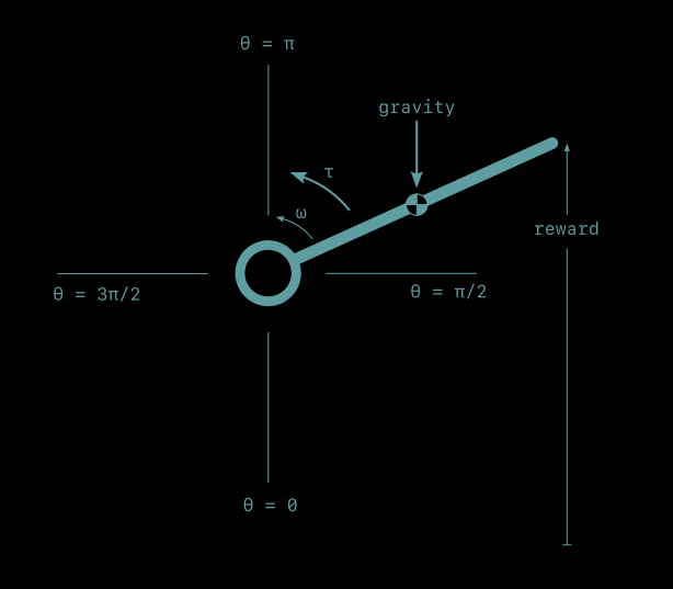
This is different from the popular cart-pole task where the base of the pendulum slides back and forth on a rail. This post considers a fixed-based pendulum, a straight arm with a pinned shoulder.
The pendulum in motion at 8 frames per second, the frequency at which the agent gets updated on the pendulum's sensors and issues new action commands.
Physics
The physical representation of the pendulum is simplistic. The arm has uniform mass. It has a small amount of rotational friction, proportional to its speed. And gravity acts on the pendulum's center of mass, pulling it downward.
As always, the canonical source of information is the code itself.
Sensors
There are two quantities returned by sensors: pendulum position and rotational speed.
Position, θ, is measured in radians, zero when pointing straight down, θ = π/2 when pointing to the right, θ = π when pointing upward, and continuing around to almost 2π when it reaches the bottom again and resets to 0.
Angular speed, ω, is measured in radians per second. Positive angular speed is counter-clockwise (the direction of increasing position) and negative speed is clockwise.
Actions
Actions take the form of torque, τ, applied to the base of the pendulum. Positive torque accelerates the pendulum counter-clockwise, in the direction of increasing position. Negative torque accelerates it in the clockwise direction.
Actions are discrete in time. Each action is a constant torque that lasts for 1/8 second.
There are 13 discrete values the torque can take, 6 positive, 6 negative, and zero. Possible torque values are distributed nonuniformly across the range, with the middle half of the range having denser coverage. This results in a finer grained representation of small torques, useful for making fine-tuning adjustments.
Reward
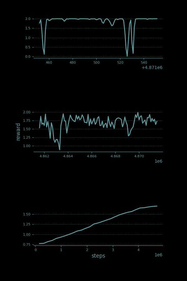
The pendulum returns reward, r, related to how high the its swinging end reaches, its vertical distance from its straight down θ = 0 position. It reaches a maximum of r = 2 at the straight up θ = π position. A successful learning curve will work its way up to 2 and stay there.
Three traces of reward collected by a spinning pendulum at 8x real time, covering short, medium, and longer term history.
Cheat mode: Servo
We can skip every hard and interesting part of this problem by using a servo, a motor and controller that take a desired position and drive the pendulum arm directly to it. It hides the problem from us. Instead of taking torque as an input and generating motion as an output, a servo allows us to provide the final answer, and then tells us not to look behind the curtain while it solves the problem for us. This is usually done by gearing the drive motor down so far that the pendulum dynamics become easy to ignore or by implementing some kind of controller in a black box.
The servo solution is worth mentioning because it's common. When working with a machine that’s big enough to hurt when it hits you, it’s nice to know exactly where it’s going to be and when. This is one of the reasons that reinforcement learning is not frequently used in robots. (But also something I would love to change.)
Level 1: Bang-bang control
One of the most straightforward ways to control a pendulum is to sense whether it is to the right or to the left of its desired position and apply the maximum torque the other direction. For some systems this works remarkably well. It’s also straightforward to implement. There’s no math other than a comparison with the desired position.
Bang-bang control does require knowing a fair amount about your system, though.
- It requires knowing which position is the desired position. In a pendulum, the connection between position and reward is clear, but in real systems, it can be quite complex. In robots, it’s likely to involve the positions and velocities of many degrees of freedom, and probably their time histories as well.
- It requires knowing how the current state is related to the goal state In the pendulum, it’s obvious that θ greater than π is past the goal in the counterclockwise direction while θ less than π is past the goal in the clockwise direction. The relationship of every pendulum position to the goal is straightforward. This isn’t always the case. Driving through the crisscross of one-way streets that is downtown Boston demonstrates how the appearance of being close to a goal may not reflect the realities. The distance as the crow flies is only very loosely related to the actual driving distance, which itself is only a very approximately connected to the drive time.
- It requires knowning which action will drive the system closer to its goal. Again in the pendulum this is obvious, but even in systems with two degress of freedom the connection becomes less obvious quickly. Assuming that we know which actions drive a system to its goal is a big assumption.
Bang-bang control in a pendulum, while effective, only works because it allows us to build in a lot of implicit knowledge about how a pendulum works.
Level 2: PD control
Bang-bang control is inelegant. When driving a car, bang-bang control would be having the accelerator fully depressed until you reach your destination, at which point you instantly slam it into reverse. It can be hard on your machine and on any humans involved. It can also result in poor performance, overshoot of the goal, and an audible "bang" when actuators switch instantly from full speed ahead to full reverse.
A useful improvement over a bang-bang is proportional-derivative (PD) control. It gets around some of the more obnoxious shortcomings of bang-bang control by adjusting its torque appropriately. The further away the pendulum is from the goal, the greater the torque applied to move it back (proportional control). And to help keep it stable, a small torque is added in the direction opposite to that of the pendulum's movement, simulating friction (derivative control).
Similarly to bang-bang control, PD-control drives the pendulum directly to its target position, albeit less violently. And like bang-bang control, it requires knowing which pendulum state maps to maximum reward, where pendulum states are relative to each other, and which actions move the pendulum from its current state to the goal state.
Level 3: Q-learning
The difficulty level goes up considerably if we take away knowledge about which position is rewarded, where the current position is in relation to it, and which action will move the system closer to its goal. This is the difficulty level on which Q-learning operates.
Rather than working with continuous angular positions and velocties, Q-learning works with a discretized state representation. Position is chopped into discrete bins, as is velocity. Now, instead of θ being able to take on any real value between 0 and 2π, it has a relatively small number of discrete options to choose from. Similarly with ω. And because there are just a handful of positions and velocities to choose from, we can list every possible combination of them, together with every action that can be taken, in one big table. Then, learning to control the pendulum becomes a task of filling in the table—of trying every action in every state a few times and learning what reward tends to occur.
This takes a while but it does eventually happen.
Level 4: Q-learning with curiosity
Q-learning is a classical reinforcement learning technique. It relaxes all the assumptions and system knowledge required by PD or bang-bang control. It does the job, but very slowly. The reason it is so slow is ε-greedy exploration. At the very beginning of its life the agent has no idea which actions are the most lucrative in any given situation. Even so, it only spends a few percent of its time exploring. And after millions of trials when it knows very well what to do, it still spends a few percent of its time exploring, which prevents it from getting very close to perfect behavior.
An alternative is exploration based on curiosity. There are many different ways to describe and implement curiosity, but my favorite is one I rolled myself. It assigns an explicit reward value to the knowledge gained from trying something new. If an action has never been tried before, uncertainty is high and it has a lot of potential value. There might be a pony behind that door you've never opened. But by the time an action has been tried seven times with the same result, it's unlikely that trying it an eighth time will give a different result. You can keep pressing the "walk" button but it's probably not going to change the light.
In this implementation of curiosity, the uncertainty associated with taking an action in a given state is related to how many times that action has been tried in that state already. More experience means lower uncertainty. Uncertainty gets collected over time as curiosity about taking that action. Once that curiosity exceeds the expected rewards of other alternatives, the agent tries that action again, and the curiosity gets reset to zero.
This results in a whole lot of exploration when the agent is young, but settles out quickly after every option has been tried a few times. It also means that, for a given state, once a very successful action is found others are much less likely to be experimented with.
A Q-learning agent that uses a curiosity strategy for exploration learns much faster than from ε-learning.
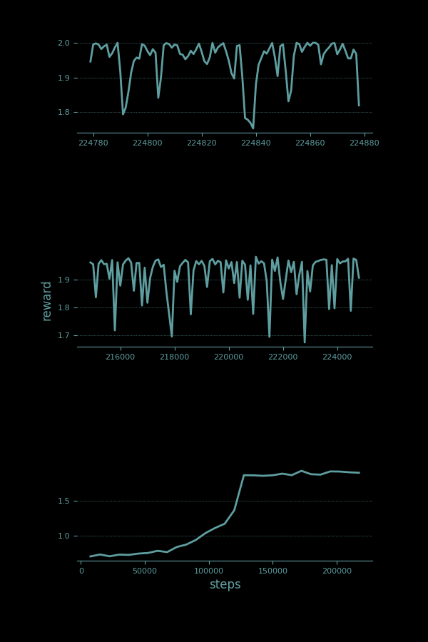
After 125K samples the pendulum settles into mostly upright position, with occasional deviations as a long tail of exploratory actions play out.
Curiosity doesn't eliminate any of the assumptions made about the system, but it does level up the performance.
Level 5: Model learning FNC
It's also possible to level up Q-learning. Q-learning updates its value function, the expected return from any state-action combination, by a small fraction each time. The same action would need to performed at least a dozen times in a given state before the learned value of that action gets close to the actual expected reward.
But there is no need to be so cautious at first. Initial learning rates can be very high. It's reasonable to assume that whatever happens the first time an action is tried in a situation will happen every time, (a learning rate of 1). Then for the second action the learning rate can be backed off, say to 1/2. This learning rate backoff continues for the third, fourth and subsequent trials, until eventually it settles in to some steady state learning rate floor, say 0.03.
A method called Fuzzy Naive Cartographer uses this trick to learn state-action values more quickly. It is an approach I developed to learning state-action-state transition world models, but it also learns a state-action-reward value function. It uses both aggressive early learning rates and curiosity-driven exploration to invert the pendulum in about 65,000 time steps.
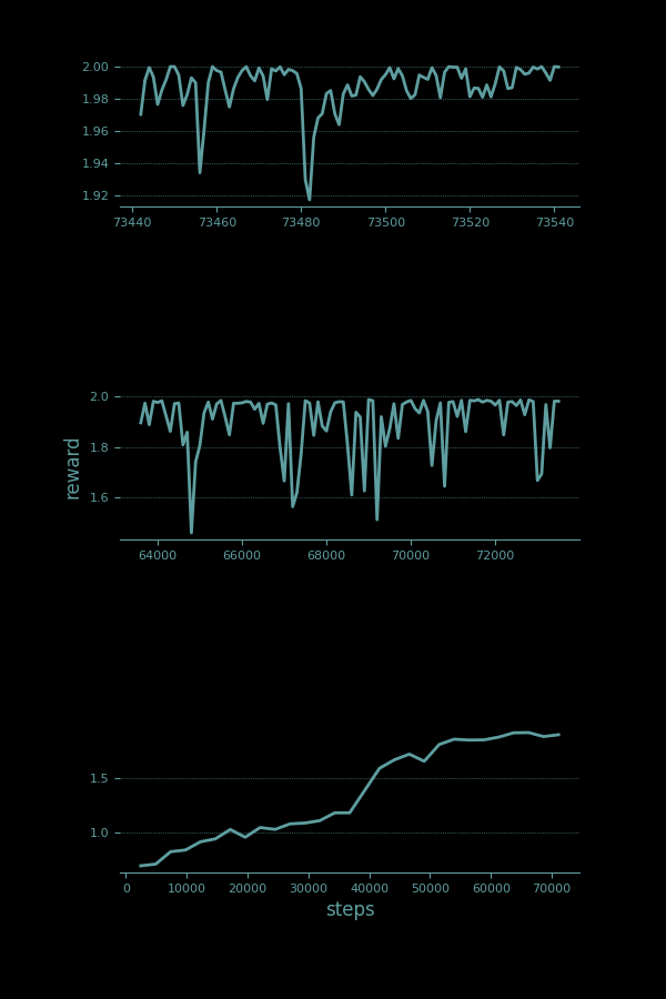
Importantly, the gains that come from adding curiosity and aggressive early learning rates do not require any specific domain knowledge or assumptions. There is no subtle pendulum understandings built into these tricks. They apply equally well to any world.
Level 6: Feature learning with Ziptie
We do however have some world-specific knowledge built in to how the state information is constructed. Each position value is paired with each velocity value to create the whole set of unique states. This seems like a very small step, and hardly any contribution of domain knowledge for the pendulum, but for systems with a large number of inputs, like an array of pressure sensors or an image with thousands of pixels, the full list of every possible combination would be imposibly large. When this is the case, small collections of sensors—a group of active pressure sensors here or a group of pixels forming a visible edge there—is a much more useful set of features to learn from.
When these combinations of sensors are designed by a human, that's called feature engineering, but when they are learned by an algorithm, that's feature learning. Feature learning allows features to emerge from the patterns that occur in the data itself, and do not rely on the intuition and biases of a designer.
The Ziptie algorithm is developed to solve exactly this problem. In the case of the pendulum, Ziptie takes in all the discrete pendulum positions and all the discrete velocity values and learns to pair every position with every velocity. It's not really necessary to do this for a system as simple as the pendulum, but automatic feature creation is a way to make the learning approach more agnostic to the world it is learning to navigate.
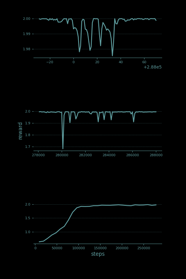
This is the first step at which we've had to make a tough trade-off. Intentionally including fewer assumptions (how state features should be constructed from raw sensors) makes the algorithm's job harder. It has an extra level of structure to learn. Before it can even start dialing in the optimal actions to take in each situation, it first has to learn to recognize those position-velocity pairs that represent each situation. The win is that the method is a lot stronger, more general. It requires less built in knowledge. The cost of this win is an extra forty thousand time steps before performance gets close to optimal, and the pendulum spends most of its time facing straight up.
This is exactly the trade-off this work is targeting. Playing on hard mode is not about learning to invert a pendulum. We've already seen there are easier ways to do that. The goal is to be able to learn to control systems that we don't know much about. Systems that are more complex or difficult to model. That's where the real power is—not in learning to do one thing better than everyone else but in learning to do more things at a B- level.
At this stage, it is helpful to note that FNC also lets go of a common assumption, that every sensor observation at every time step is relevant. Methods like Q-learning that list all possible states in a table use a dense state representation—for two states to be the same, they both must have the same value of every sensor. If there are noisy sensors present that have no bearing on what action should be taken, they will confuse the algorithm. It will fail to learn from its experience because every experience will appear completely new. FNC avoids this be treating each sensor value individually. Once it learns the best torque to apply given a position/velocity combination a hundred other irrelevant sensors won't prevent it from applying that knowledge. Combined with Ziptie, FNC learns a minimal reduced-state representation that is just rich enough to allow it to achieve its goals. This capability in FNC is rare, if not unique, among RL approaches.
Hard mode: Discretization learning with BucketTree
Even though Ziptie does a good job learning to build features, it still relies on position and angle measurements that have been carefully discretized. A lot of domain knowledge goes into designing a good discretization.
- How many discrete angle bins should there be?
- Should angle be uniformly sliced?
- Or should it be divided more finely in the neighborhood of the twelve o'clock position, to help it make the fine adjustments necessary to keep the pendulum vertical?
- How many discrete velocities?
- Should they be uniform or more densely divided near zero?
- What are the largest velocities likely to be observed?
When I was writing this world I had to do a lot of trial and error to find a discretization that was feasible to learn.
The next level of difficulty is to take away the designed discretization, to just feed raw floating-point numbers as inputs and let the discretized bins be learned automatically. This is where BucketTree comes in.
BucketTree is a tree of buckets. The root bucket contains all the values from minus infinity to plus infinity. The next level is split into two buckets, with one bucket covering minus infinity to the split, and the other covering from the split to plus infinity. And this continues for as many levels and buckets as the tree is allowed to create. A BucketTree with n full levels will have a total of 2^n - 1 buckets. The total number of buckets allowed is specified at BucketTree creation.
This process also takes time. BucketTrees learn how to divide and subdivide buckets by collecting observations. They also take care not to jump the gun and create all their bins prematurely (say, in the neighborhood of the six o'clock position of the pendulum) before they have had a chance to explore their world a little bit.
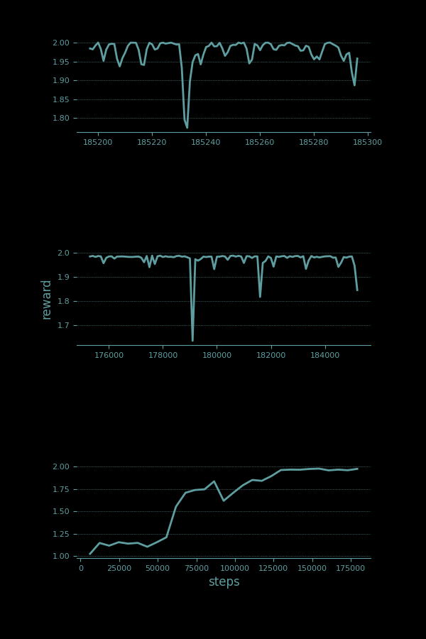
For the pendulum and its two continuous variables, learning a discretization adds an extra forty thousand time steps to its learning process.
The bins that are created for each variable seem like a reasonable representation of the space. With a maximum of 50 bins allowed for both position, θ (sensor 1, on bottom), and velocity, ω (sensor 0, on top), here's how they got bucketed.
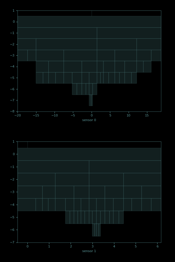
These plots show the hierarchical bucketing of each sensor. The root bucket (level 0 in the plot) covers everything from infinity to minus infinity. The next level (level -1 in the plot) has a single split, giving two child buckets. Level -2 has 4 buckets, level -3 has 8, and so on. The buckets in a single level are approximately evenly spaced, but not exatly so. In both cases, the sensor ranges closest to the reward state (θ = 3.14, ω = 0) are where it spends most of its time, and so they get subdivided into finer and finer buckets.
Notably this doesn't slow the learning down very much. This is probably because the original, hand-designed discretization (equally spaced position bins and semi-regularly spaced velocity bins) is denser than it needs to be, particularly in regions far from the reward, resulting in a larger state space.
But way more important than this, BucketTree means that the agent doesn't care whether the sensors in the world are discrete, continuous, or some of both. Whatever the case it will learn to handle it. This is in contrast to every other RL framework where you have to specify whether each sensor is continuous or discrete and give the range of each. It removes a whole stack of assumptions and domain knowledge that the vast majority of approaches require.
Harder mode: Real-time
Another assumption that many RL implementations make is that they have all the compute time they need. Some approaches are quite computationally expensive and can take a while for the agent to process all its sensor information, evaluate its options, choose its next step, and update all the paramters it is learning. During the time it takes to do this, the world spins on. Motors are still driving, limbs are still swinging, obstacles are still coming up fast. Agent processing time gets experienced as a delay. Every action the world receives is based on sensor information it sent in the past. Things have changed since then and what was the ideal action then may no longer be.
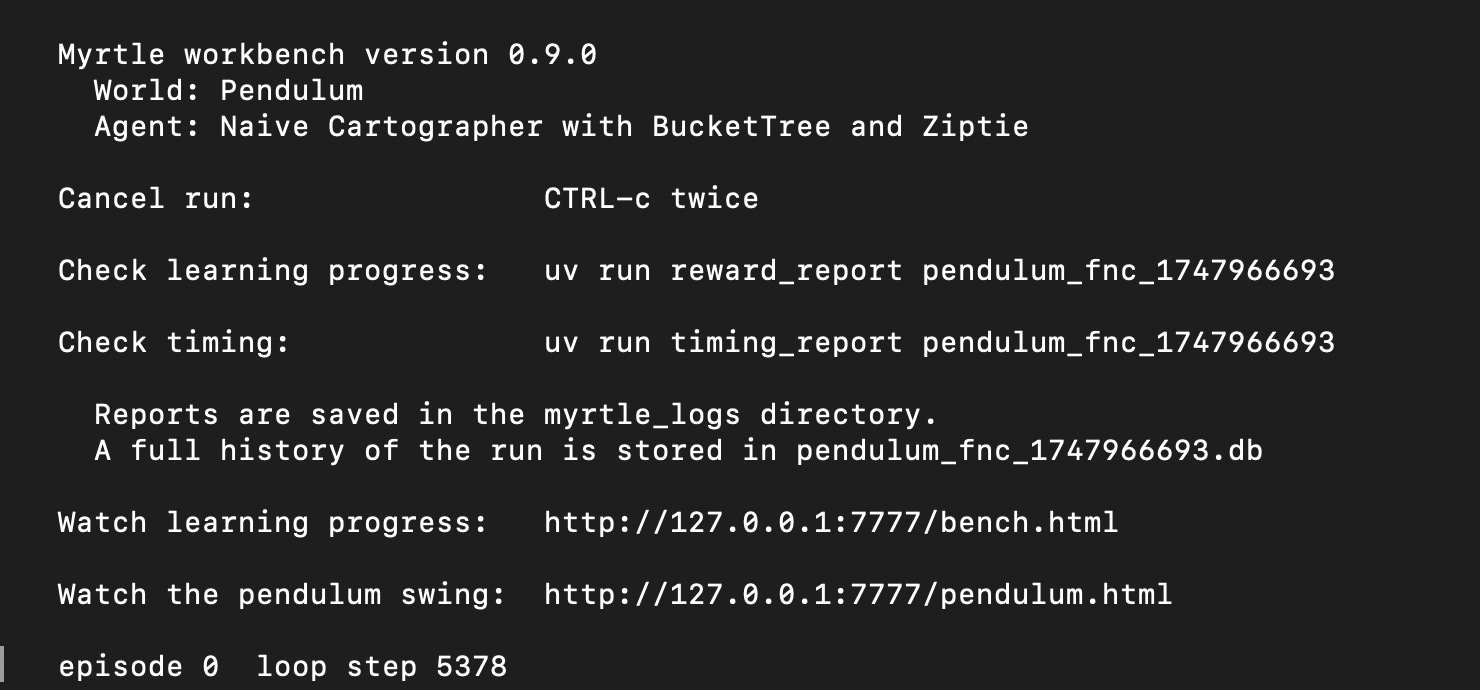
This is the challenge of operating in real-time, grounded in a wall clock. The whole pendulum exercise above has been completed with this real-time constraint in force. I created the RL workbench Myrtle to do exactly this.
Myrtle enforces real-time constraints by separating the world (the pendulum) and agent (the learning algorithm) into separate processes. This allows them to avoid blocking each other and to each use their own CPU core for processing so they don't starve each other for compute. Every other support function within Myrtle, like logging, reporting, and serving browser animations, is performed in yet another process, so that occassionally demanding processing steps don't cause hiccups in the critical processes.
The world is the metronome for the RL loop. It sends sensor information at a consistent pace thanks to a Pacemaker, a precision timekeeping tool. Although the pendulum in these examples is simulated, that simulation is also tied to the wall clock. A high speed pacemaker is used to govern the fine timesteps of the physics simulation behind it.
When working against the wall clock, it's helpful to measure how long all the different parts of the cycle take. And it's helpful to measure that over many cycles, because it will be slightly different each time.
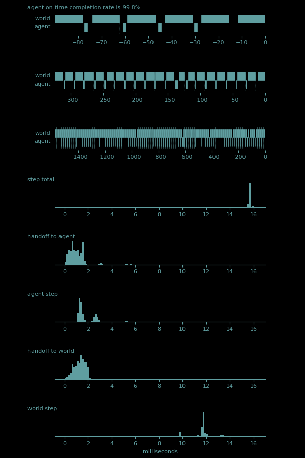
The top plot shows the most recent few cycles in the RL loop, extending from the current time, 0 ms, back to almost 100 ms ago. The bars show phases of the cycle. The world bar shows the period between when it receives an action and when it passes the next round of sensor information back to the agent. In a perfectly fast RL system, the world bar would be solid across cycles, with zero agent processing delay. In a real-time system this will never be the case. But in this plot, it shows that the world bar covers about 80% of the cycle, which is pretty good. It also shows the agent processing time. Even for the BucketTree/Ziptie/FNC stack, this is quick, a couple of milliseconds. Note that the most recent agent bar is missing. This is due to the small delays incurred in the logging process. It hasn't been recorded yet. A fine dotted line marks the end of each world bar. This is the demarcation of a new cycle. The sending of new sensor information to the agent occurs on time, regardless of any delays that came before. The gaps between the agent and world bars are the handoff times. Sensor and action information are passed using Python's multiprocessing Queues, which are quite fast, but the information still has to wait to be read by the recipient. Both the world and agent check for new information on a regular cadence. It's quick, but the letter sits in the mailbox for a few hundred microseconds.
The second and third plots are identical to the first, except that they cover more and more cycles. This gives a chance for different patterns and anomalies to become visible.
The fourth plot shows the distribution of the time per cycle. The pendulum control loop is running at 8 cycles per second. Given the physical dynamics of the pendulum, issuing motor torque commands 8 times in a second is the sweet spot for being able to control it well. Much faster than that and the effect of an action is hard to observe. Much slower than that and the pendulum can swing way past where you wanted it to go. Because I am impatient, the whole system is also running with an 8x speedup. That means that it's able to squeeze 64 cycles into a second while faithfully simulating the dynamics of the 8 cycle per second contol. As a result, the total cycle time ends up being 1/64 seconds, or 15.6 milliseconds. This plot demonstrates how carefully Myrtle is able to maintain that cadence, with a sharp peak at 15.6.
The fifth through eighth plots break down this total cycle time into its pieces
- the handoff from the world to the agent (the gap between the world bar and the agent bar)
- the agent step time (the length of the agent bar)
- the handoff from the agent to the world (the gap between the agent bar and the world bar)
- the world step time (the length of the world bar)
As expected, these distributions visually add up to the total cycle time. What may not be expected is the structure of these. Handoffs show a central tendency, but with a wide smear. Agent step is bi-modal, probably showing large processing steps that occur during some iterations and not others. And all the plots show small regularly spaced bumps, indicating that sometimes things just take longer than expected, and when they do it's usually by about 2 ms.
Bonus points: Simple reward function
It's a minor point, but worth mentioning: Myrtle's pendulum is also using a simpler reward function than the widely used Gymnasium pendulum. Gymnasium as a fantastic resource with a wide variety of worlds for a RL agent to try themselves against. The implementation of the Gymnasium pendulum has a reward that includes a stiff penalty for moving quickly, as well as a cost for taking large actions.
-(θ^2 + ω^2/10 + τ^2/1000)
(Note that θ in the Gymnasium pendulum is defined as zero in the upright position, positive to the right and negative to the left.)
This formulation gives indirect hints to the agent about what strategies it should adopt. It directly penalizes wild swings and hard twists. It's not wrong to do this, but it is important to note that the reward function is a common place for domain-specific knowledge and assumptions to get baked into the algorithm. Removing these extraneous terms, as we have, makes learning to control the pendulum a greater challenge. Definitely worthy of some bonus points.
Next level
There are some remaining parts of the system that are either assumed away or hard coded. To get to a truly general solution, operating on ultimate, no cheat-codes hard mode, I'll need to find a way for the RL agent to learn all of these.
Action discretization
The set of discrete actions available to the agent is extremely hard coded. The list of torque values was developed through trial and error and the learnability of the world is sensitive to them. BucketTree is great at automatically discretizing sensors, but the problem of learning useful action discretizations is a tougher one. I'm uncomfortable having this much hard-coded domain knowledge in the world. It is an itch in my brain. It is on my to-do list to make this learnable as well.
Time discretization
The cadence at which the world-agent RL loop runs is another magic number, chosen through trial and error, and the learnability of the world depends on it heavily. The representation of time is even more fundamental than representing actions. How we choose to discretize time has a profound effect on how agents and worlds can interact. It would be wonderful to be able to learn a good discretization.
There is precedent for this. In numerical integration, the Adaptive Runge—Kutta method runs multiple estimates of a dynamic system at different orders, and it adjusts the time step so that the error differences between those lower- and higher-order estimates stays in a given range. I still haven't worked out how to apply this concept to RL, but it is also on my to-do list.
Sequences and time-series
For many systems, it's not only the current set of sensor values that determine what the next action should be, it's also the recent history of them. Imagine a pendulum that has only a position sensor, but no velocity. The velocity is important to know when deciding how much torque to apply. While it can't be measured exactly in the position-only pendulum, it can be estimated by looking at the last few positions and action torques.
The methods described here all assume that the current set of observations are all that's needed for deciding the best action to take next, also called the Markov Assumption. To become more general and play on yet harder levels, it will be necessary to relax this assumption. This is something I'm working on currently.
Dealing with sequences is likely to require some form of attention, focusing on some sensors while ignoring others. The possible combinations of sensor values grows exponentially with the number of time steps included in the history. Attention is a way to filter down the sensor values to the most relevant ones, keeping the problem tractable.
Hyperparameters
So far I've conveniently avoided the fact that even when algorithms like Ziptie and BucketTree learn to sidestep hard-coded domain knowledge, they still have a few hard coded parameters of their own that govern their behavior. For both of them it's important to choose the right capacity—the maximum number of features that Ziptie can create and the limit on the number of buckets that BucketTree can create. There are also thresholds that determine how quickly new features and buckets get formed.
Learning discretizations and features involves a certain amount of kicking the can down the road. Even though I'm no longer hard coding pendulum-specific information, I'm still hard coding the behaviors of the algorithms that learn them, their hyperparameters. But while the algorithms' performance is quite sensitive to their hyperparameters, they can learn a broad swath of systems, far more than just a single degree of freedom pendulum. Learning the features of a system and learning the discretization of its inputs make this approach applicable to far more systems than it would be without them. If there are still a few magic numbers to choose, then that's a small price to pay.
The process of choosing those magic numbers, hyperparameter optimization, is a popular machine learning topic. Typical approaches range from sophisticated Bayesian algorithms to simply trying everything. But by far the most common approach is researchers trial-and-erroring their way into something that works pretty well most of the time. This isn't a terrible way to go. Often the hyperparameters have specific meanings, and the mental models of the researchers let them intuit their way into good values much faster than could be discovered by brute force.
Bayesian hyperparameter optimization falls on the side of improving performance by building in more domain knowledge (known in Bayesian circles as priors). Exhaustive search falls on the other side. It's horribly inefficient, but assumes nothing about the way hyperparameters act or interact. A middle ground can be found in Evolutionary Powell's method, a method I created to randomly explore the hyperparameter space, but in a way that is weighted toward the most successful runs seen so far.
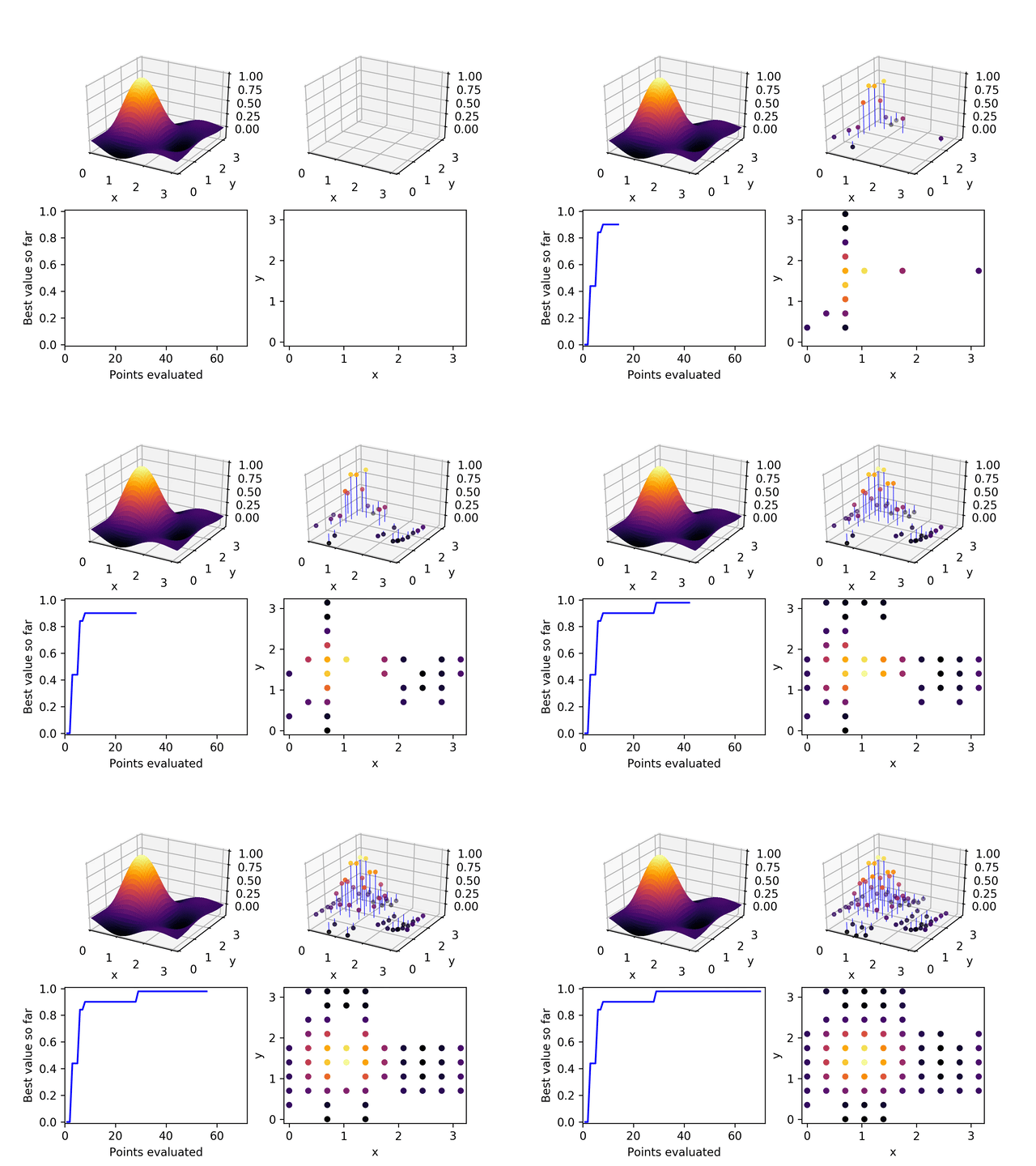
In this animated example the exploration proceeds along one dimension at a time (in the spirit of Powell's method but the selection of the starting point for each new dimension is weighted according to the performance of its nearest evaluated neighbors.
I didn't set up hyperparameter optimization for these examples, but this is the path I would use to avoid making assumptions and hard-coding hyperparameters
How far can this go? How assumption-free can we get?
A loosely related concept here is the No Free Lunch Theorem. In a gross oversimplification, it states that if algorithm A performs better than algorithm B on a task, there is another task for which the reverse will be true. There is no algorithm which performs better on every possible problem. The best you can do is identify the set of problems you care about the most and look for algorithms that perform well on them, at the expense of all the others. In the case of controlling robots, we can definitely do this. We don't need an approach that can learn to maximize reward on just any system. There are a handful assumptions we can focus on,
- physical systems and simulations of physical systems,
- with length scales from a few millimeters to a few meters,
- on time scales from a few milliseconds to a few days,
- that are dominated by classical mechanics.
Although this is a huge class of systems, it is an infinitessimal segment of all possible control problems. This is good news. It means that even with the No Free Lunch Theorem in effect it's conceivable to develop learning approaches that perform pretty well across most of them. Which is exactly what controlling a pendulum on hard mode is trying to do.
Ziptie, BucketTree, and FNC minimize the amount of problem-specific engineering that needs to be done. They get us closer to the ultimate goal of a domain-agnostic RL agent, a plug-and-play robot brain.
Appendix: Running the examples
1) Download the code
git clone https://codeberg.org/brohrer/pendulum-examples.git
cd pendulum-examples
2) Download uv if you don't already have it
curl -LsSf https://astral.sh/uv/install.sh | sh
3) Choose an example and run it
uv run buckettree_ziptie_fnc.py
